My research group has compiled a dataset that counts the number of cases of Sudden Unexpected Infant Death (SUID) in each census tract of Cook County, IL from 2015-2019. We want an accurate way to estimate the risk of SUID in each tract using this data. SUID is defined as any case of death in a baby less than age 1 year old that does not have a known cause before a medical autopsy is performed. While the state of Illinois releases statistics about SUID for the county as a whole, we think it’s important to understand this phenomenon at a more granular geographic level. That way, we have a better understanding of geographic disparities and service agencies can more precisely target their interventions.
The goal of this post is to convince you that Bayesian techniques offer a more principled way to estimate a risk process when the amount of observed data has limitations by itself.
Intro to the Data
Here’s what our dataset looks like:
library(tidyverse)library(leaflet)suid_base_table <-read_csv(here::here("data", "suid_snapshot_2022_08_31.csv")) |># Remove rows with NA values for count of SUID cases or for population under fivefilter(!is.na(suid_count) &!is.na(pop_under_five)) |>select(fips, suid_count, pop_under_five)suid_base_table
Each row is an individual census tract. The fips column lists each tract’s unique identifier, suid_count is the number of SUID cases that took place from 2015-2019, and pop_under_five is the population of children under age five as estimated by the U.S. Census’ American Community Survey.
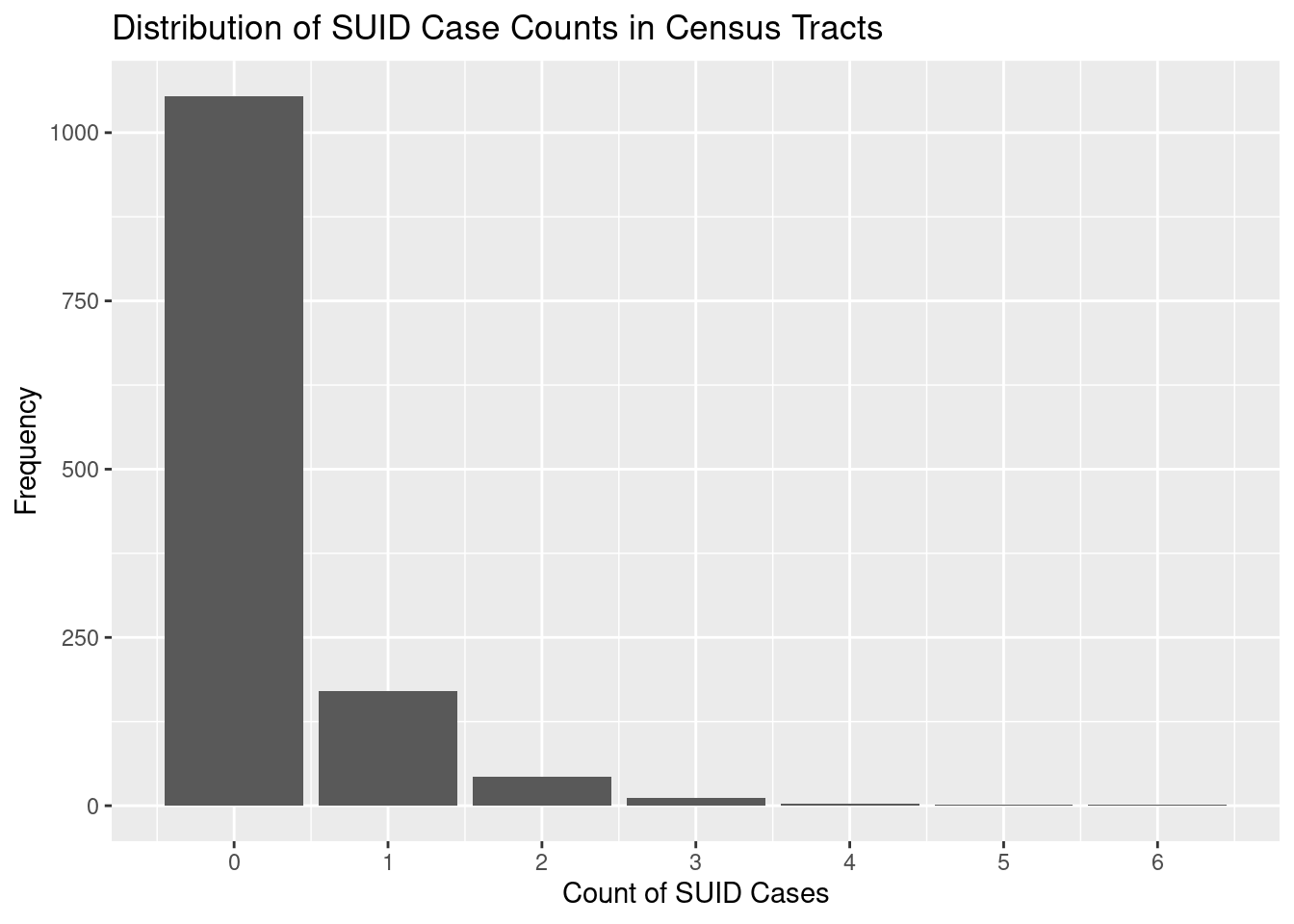
It’s important to note that SUID is a rare event. The vast majority of census tracts did not suffer any cases of SUID during this time period. Here’s a histogram to illustrate:
The first challenge in estimating the risk is we don’t have the proper denominator. SUID incidence is typically reported as cases per 100,000 live births. However, we don’t have disaggregated counts of live births in each census tract. The best approximation I have found is pop_under_five, which I hope reasonably mirrors the number of live births over a five-year period. Here are approximated incidences for each tract using pop_under_five as denominator:
That’s also not what we were looking for. What’s going on?
A problem that emerges from using pop_under_five as the denominator is that five tracts are estimated to have zero children under the age of five. In such cases, R calculates the incidence as NaN (not a number) when suid_count is zero and as Inf (infinity) when suid_count is anything greater than zero:
suid_incidence_table |>filter(pop_under_five ==0)
# A tibble: 5 × 4
         fips suid_count pop_under_five suid_incidence
        <dbl>      <dbl>          <dbl>          <dbl>
1 17031081000          0              0            NaN
2 17031280800          0              0            NaN
3 17031380200          0              0            NaN
4 17031670100          1              0            Inf
5 17031834900          1              0            Inf
We know that the true risk for these tracts can’t be a non-existent number or infinitely large, so we’ll do our best adjust for these circumstances:
suid_incidence_table <- suid_incidence_table |>mutate(suid_incidence =case_when(# If incidence is NaN, change to 0is.nan(suid_incidence) ~0,# If it's Inf, change to 100,000is.infinite(suid_incidence) ~1E5,# Otherwise, keep as isTRUE~ suid_incidence ) )
Now let’s try and calculate the mean:
mean(suid_incidence_table$suid_incidence)
[1] 339.1101
A much more sensible number, although it still seems like an overestimate compared to the overall incidence for Cook County, which is 88.3 cases per 100,000 births per Illinois Department of Health.
Let’s take a look at the census tracts with lowest and highest incidences:
On both extremes, the incidence values seem intuitively implausible when used to characterize the underlying risk for SUID. On one end, we shouldn’t expect that a tract’s risk for SUID was zero just because there were no observed cases. SUID is rare, so it’s expected that many tracts will count zero cases just by luck of the draw.
On the other end, notice how the tracts with highest incidence of SUID also tend to have low populations under five. Let’s take an aside for a minute and think about flipping a coin and using the results to estimate whether that coin is weighted to favor a certain side. If you flip a coin three times and get heads every single time, do you think it’s actually weighted to favor heads? What about if you flip it 500 times and still get heads every single time? You should be a lot more confident after 500 coin flips that the coin is truly weighted because you’ve accumulated more evidence. Similarly, think of every live birth as a coin flip that accumulates evidence about the underlying risk of SUID. The more live births there are, the more confident we can be that the observed incidence matches the true risk for SUID. Said another way, census tracts with high incidence but low counts of pop_under_five might just be very unlucky, rather than truly at higher risk.
Given these limitations of approximating incidence, we are going to use a Bayesian approach to adjust estimations to incorporate our “prior” expectations of what the underlying risk process should look like.
Step 1: Set your prior expectations
We are going to use the “Beta distribution” to represent our prior expectations. The Beta distribution is not nearly as well known as others like the normal distribution (aka Bell Curve), but the Beta is particularly well suited to represent a plausible values for a risk process. Check out David Robinson’s post here for more explanation. The Beta distribution has two “parameters”. The number of observed events is represented by \(\alpha\) (SUID cases) and the number of trials that don’t result in an event is represented by \(\beta\) (live births that don’t result in SUID, aka survivals). Let’s try using Cook County’s overall incidence of SUID and count of live births to set our prior expectations:
# Sourced from Illinois Vital Statistics# https://dph.illinois.gov/topics-services/life-stages-populations/infant-mortality/sids/sleep-related-death-statistics.htmloverall_incidence <-88.3/1E5# per live birth for Cook County in 2014overall_incidence
[1] 0.000883
# https://dph.illinois.gov/data-statistics/vital-statistics/birth-statistics.htmltotal_live_births <-139398# for Cook County from 2015-2019extrapolated_cases <- overall_incidence * total_live_birthsextrapolated_cases
A cool thing about the Beta distribution is it will adjust it’s shape to reflect the number of observations (aka evidence) we give it. I’ll try and illustrate by rescaling the parameters to reflect the relative number of live births (coin flips of evidence) in the county versus in a typical census tract.
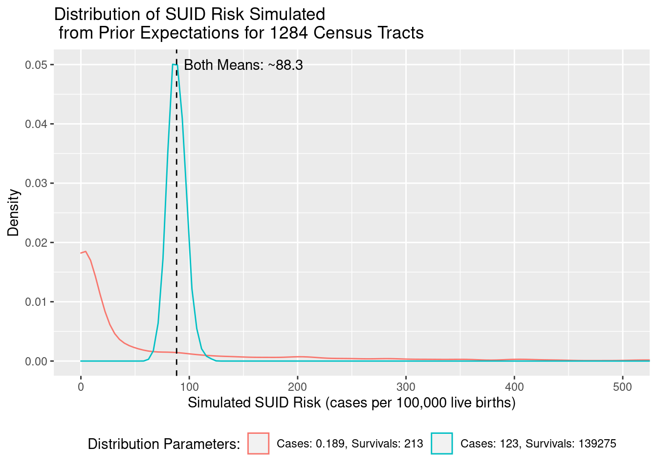
Let’s simulate two Beta distributions of 1,284 census tracts. One will use parameters reflecting the amount of evidence accumulated for a whole county’s worth of live births, versus just a census tract’s worth of live births.
Both distributions have the same ratio of cases (\(\alpha\)) to survivals (\(\beta\)), so their mean expected SUID Risk is about the same at 88.3 cases per 100,000 live births, but the blue distribution observed a county’s worth of live birth evidence (139,398), so its range of expected values is much more compact (about 70 to 120) than a census tract’s worth of live birth evidence (estimating risk anywhere from 0 to 500).
In Bayesian analysis, we combine our prior expectations with observed data to get a “posterior” estimate. In this case, I want the prior expectation to weigh about the same as the observed data, so I’ll use census-tract-scaled parameters in my prior.
Step 2: Combine the prior expectation and observed data
To get each posterior estimate of risk from the Beta distribution, we are going to perform the following calculation:
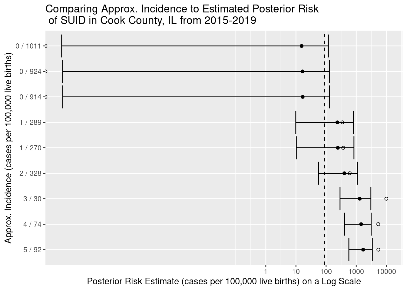
Let’s visualize how our posterior estimates of risk relate to incidence calculations and prior expectations:
On the Y axis, we have 9 census tracts for which we’ve estimated risk. We label each tract with the observed data used to calculate approximate incidence. For example, the top row shows a census tract that observed zero cases of SUID and had a population under five of 1,011 children. Each approximate incidence is marked on the x axis as a hollow circle for reference. Each filled black circle marks our posterior estimate of SUID risk and is flanked by a 95% credible interval (the Bayesian cousin to the confidence interval). The dashed vertical line marks our prior expectation of risk as observed for the whole county.
What I want you to notice is how the posterior estimate represents a tug-of-war between the prior expectation (dashed line) and the observed data (hollow circle). The prior expectation is able to pull our estimates away from extreme observed incidence values (like 0 in the top three rows, or over 5000 in the bottom three rows) to more plausible values. This balance between the forces of expectation and observation is what makes Bayesian estimation so powerful!
Geographic Pattern?
When we map census tracts with the 100 highest and 100 lowest estimates of SUID risk, we notice a pattern starting to emerge. The lowest estimates are concentrating on the West/South sides of Chicago and the Southern suburbs. These areas are where historic trends of segregation have caused concentration of socioeconomic vulnerability. When you think about it, we might expect these areas to have higher risk of SUID even before we observe the data. In a future blog post, I’ll show how we can use auxiliary information about tracts (like location or SES) to fine tune our prior expectations of risk for a better posterior estimate.