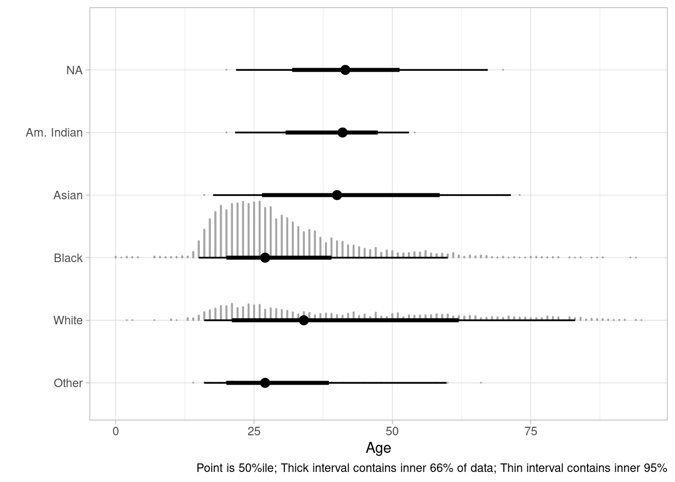
Characterizing Age of Victims of Gun-Related Deaths in Cook County, IL, 2017-2021

guns
epidemiology
Author

Daniel P. Hall Riggins, MD

Published

October 2, 2022

Set-Up

Data was sourced from the Cook County Medical Examiner’s Office and modified according to the data pipeline in this commit of my Github repository.

Code
library(tidyverse)
library(lubridate)
library(ggdist)

theme_set(theme_light())

# Parquet file generated from the ccme_archive_generic target in data pipeline linked above
ccme <- arrow::read_parquet(here::here("data", "ccme_archive_generic_2022_10_02.parquet"))

gsw_deaths <-
    ccme |> 
    filter(gun_related == TRUE) |> 
    filter(death_date > ymd("2014-12-31") & death_date < ymd("2022-01-01")) |> 
    mutate(
        manner = factor(manner, levels = c(NA, "SUICIDE", "HOMICIDE", "ACCIDENT"), ordered = TRUE),
        race = factor(race, levels = c("Other", "White", "Black", "Asian", "Am. Indian", NA), ordered = TRUE)
    )

Image Source: https://www.chicagotribune.com/news/ct-viz-cta-red-line-station-shooting-20200229-uaofbvsknbfv3g4xlqph4kdudi-photogallery.html

Age Unstratified

Code
gsw_deaths |> 
    ggplot(aes(x = age)) +
    stat_dotsinterval() +
    labs(
        x = "Age",
        y = "Density",
        caption = "Point is 50%ile; Thick interval contains inner 66% of data; Thin interval contains inner 95%"
    )

Code
quantile(gsw_deaths$age, probs = seq(0, 1, 0.1), na.rm = TRUE)
  0%  10%  20%  30%  40%  50%  60%  70%  80%  90% 100% 
   0   18   21   23   25   28   31   36   42   55   95 

Age Stratified by Manner of Death

Code
gsw_deaths |> 
    ggplot(aes(x = age, y = manner)) +
    stat_dotsinterval() +
    labs(
        x = "Age", y = "",
        caption = "Point is 50%ile; Thick interval contains inner 66% of data; Thin interval contains inner 95%"
    )

Code
gsw_deaths |> 
    group_by(manner) |> 
    summarise(
        "0th Percentile" = round(quantile(age, probs = 0, na.rm = TRUE)),
        "10th Percentile" = round(quantile(age, probs = 0.1, na.rm = TRUE)),
        "20th Percentile" = round(quantile(age, probs = 0.2, na.rm = TRUE)),
        "30th Percentile" = round(quantile(age, probs = 0.3, na.rm = TRUE)),
        "40th Percentile" = round(quantile(age, probs = 0.4, na.rm = TRUE)),
        "50th Percentile" = round(quantile(age, probs = 0.5, na.rm = TRUE)),
        "60th Percentile" = round(quantile(age, probs = 0.6, na.rm = TRUE)),
        "70th Percentile" = round(quantile(age, probs = 0.7, na.rm = TRUE)),
        "80th Percentile" = round(quantile(age, probs = 0.8, na.rm = TRUE)),
        "90th Percentile" = round(quantile(age, probs = 0.9, na.rm = TRUE)),
        "100th Percentile" = round(quantile(age, probs = 1, na.rm = TRUE)),
    ) |> 
    pivot_longer(cols = 2:12, names_to = " ", values_to = "value") |> 
    pivot_wider(names_from = manner, values_from = value) |> 
    select(
        " ",
        "NA, n=39" = "NA",
        "Accident, n=10" = ACCIDENT,
        "Homicide, n=5156" = HOMICIDE,
        "Suicide, n=1064" = SUICIDE,
    ) |> 
    knitr::kable()
NA, n=39 Accident, n=10 Homicide, n=5156 Suicide, n=1064
0th Percentile 2 3 0 11
10th Percentile 7 15 18 22
20th Percentile 17 20 20 27
30th Percentile 18 22 22 33
40th Percentile 21 27 24 41
50th Percentile 24 32 27 48
60th Percentile 26 34 29 55
70th Percentile 40 40 32 61
80th Percentile 47 51 37 68
90th Percentile 59 55 45 78
100th Percentile 63 70 88 95

Age Stratified by Gender

Code
gsw_deaths |> 
    ggplot(aes(x = age, y = gender)) +
    stat_dotsinterval() +
    labs(
        x = "Age", y = "",
        caption = "Point is 50%ile; Thick interval contains inner 66% of data; Thin interval contains inner 95%"
    )

Code
gsw_deaths |> 
    group_by(gender) |> 
    summarise(
        "0th Percentile" = round(quantile(age, probs = 0, na.rm = TRUE)),
        "10th Percentile" = round(quantile(age, probs = 0.1, na.rm = TRUE)),
        "20th Percentile" = round(quantile(age, probs = 0.2, na.rm = TRUE)),
        "30th Percentile" = round(quantile(age, probs = 0.3, na.rm = TRUE)),
        "40th Percentile" = round(quantile(age, probs = 0.4, na.rm = TRUE)),
        "50th Percentile" = round(quantile(age, probs = 0.5, na.rm = TRUE)),
        "60th Percentile" = round(quantile(age, probs = 0.6, na.rm = TRUE)),
        "70th Percentile" = round(quantile(age, probs = 0.7, na.rm = TRUE)),
        "80th Percentile" = round(quantile(age, probs = 0.8, na.rm = TRUE)),
        "90th Percentile" = round(quantile(age, probs = 0.9, na.rm = TRUE)),
        "100th Percentile" = round(quantile(age, probs = 1, na.rm = TRUE)),
    ) |> 
    pivot_longer(cols = 2:12, names_to = " ", values_to = "value") |> 
    pivot_wider(names_from = gender, values_from = value) |> 
    select(
        " ",
        "Female, n=557" = "Female",
        "Male, n=5712" = "Male",
    ) |> 
    knitr::kable()
Female, n=557 Male, n=5712
0th Percentile 0 0
10th Percentile 18 18
20th Percentile 20 21
30th Percentile 23 23
40th Percentile 26 25
50th Percentile 28 28
60th Percentile 32 31
70th Percentile 38 35
80th Percentile 46 42
90th Percentile 56 55
100th Percentile 88 95

Age Stratified by Race

Code
gsw_deaths |> 
    ggplot(aes(x = age, y = race)) +
    stat_dotsinterval() +
    labs(
        x = "Age", y = "",
        caption = "Point is 50%ile; Thick interval contains inner 66% of data; Thin interval contains inner 95%"
    )

Code
gsw_deaths |> 
    group_by(race) |> 
    summarise(
        "0th Percentile" = round(quantile(age, probs = 0, na.rm = TRUE)),
        "10th Percentile" = round(quantile(age, probs = 0.1, na.rm = TRUE)),
        "20th Percentile" = round(quantile(age, probs = 0.2, na.rm = TRUE)),
        "30th Percentile" = round(quantile(age, probs = 0.3, na.rm = TRUE)),
        "40th Percentile" = round(quantile(age, probs = 0.4, na.rm = TRUE)),
        "50th Percentile" = round(quantile(age, probs = 0.5, na.rm = TRUE)),
        "60th Percentile" = round(quantile(age, probs = 0.6, na.rm = TRUE)),
        "70th Percentile" = round(quantile(age, probs = 0.7, na.rm = TRUE)),
        "80th Percentile" = round(quantile(age, probs = 0.8, na.rm = TRUE)),
        "90th Percentile" = round(quantile(age, probs = 0.9, na.rm = TRUE)),
        "100th Percentile" = round(quantile(age, probs = 1, na.rm = TRUE)),
    ) |> 
    pivot_longer(cols = 2:12, names_to = " ", values_to = "value") |> 
    pivot_wider(names_from = race, values_from = value) |> 
    select(
        " ",
        "NA, n=7" = "NA",
        "Am. Indian, n=4" = "Am. Indian",
        "Asian, n=33" = Asian,
        "Black, n=4438" = Black,
        "White, n=1742" = White,
        "Other, n=45" = Other
    ) |> 
    knitr::kable()
NA, n=7 Am. Indian, n=4 Asian, n=33 Black, n=4438 White, n=1742 Other, n=45
0th Percentile 20 20 16 0 2 14
10th Percentile 27 26 25 18 19 19
20th Percentile 34 33 28 20 22 21
30th Percentile 36 39 32 23 25 21
40th Percentile 39 41 35 25 29 24
50th Percentile 42 41 40 27 34 27
60th Percentile 44 41 45 29 42 29
70th Percentile 46 42 50 32 50 33
80th Percentile 48 46 58 37 59 37
90th Percentile 59 50 67 45 71 43
100th Percentile 70 54 73 94 95 66

Age Stratified by Latino Ethnicity

Code
gsw_deaths |> 
    ggplot(aes(x = age, y = latino)) +
    stat_dotsinterval() +
    labs(
        x = "Age", y = "",
        caption = "Point is 50%ile; Thick interval contains inner 66% of data; Thin interval contains inner 95%"
    )

Code
gsw_deaths |> 
    group_by(latino) |> 
    summarise(
        "0th Percentile" = round(quantile(age, probs = 0, na.rm = TRUE)),
        "10th Percentile" = round(quantile(age, probs = 0.1, na.rm = TRUE)),
        "20th Percentile" = round(quantile(age, probs = 0.2, na.rm = TRUE)),
        "30th Percentile" = round(quantile(age, probs = 0.3, na.rm = TRUE)),
        "40th Percentile" = round(quantile(age, probs = 0.4, na.rm = TRUE)),
        "50th Percentile" = round(quantile(age, probs = 0.5, na.rm = TRUE)),
        "60th Percentile" = round(quantile(age, probs = 0.6, na.rm = TRUE)),
        "70th Percentile" = round(quantile(age, probs = 0.7, na.rm = TRUE)),
        "80th Percentile" = round(quantile(age, probs = 0.8, na.rm = TRUE)),
        "90th Percentile" = round(quantile(age, probs = 0.9, na.rm = TRUE)),
        "100th Percentile" = round(quantile(age, probs = 1, na.rm = TRUE)),
    ) |> 
    pivot_longer(cols = 2:12, names_to = " ", values_to = "value") |> 
    pivot_wider(names_from = latino, values_from = value) |> 
    select(
        " ",
        "True, n=897" = "TRUE",
        "False, n=5372" = "FALSE",
    ) |> 
    knitr::kable()
True, n=897 False, n=5372
0th Percentile 2 0
10th Percentile 18 18
20th Percentile 20 21
30th Percentile 21 23
40th Percentile 23 26
50th Percentile 26 28
60th Percentile 28 32
70th Percentile 32 36
80th Percentile 39 43
90th Percentile 47 57
100th Percentile 84 95